As X Approaches Negative Infinity

Limits at Infinity

Limits at infinity truly are not so difficult in one case yous've become familiarized with and so, but at commencement, they may seem somewhat obscure. The basic premise of limits at infinity is that many functions approach a specific y-value as their independent variable becomes increasingly large or small. Nosotros're going to look at a few different functions as their independent variable approaches infinity, then start a new worksheet called 04-Limits at Infinity, then recreate the post-obit graph.

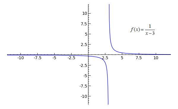
plot(1/(x-three), ten, -100, 100, randomize=Fake, plot_points=10001) \     .bear witness(xmin=-10, xmax=10, ymin=-10, ymax=10)

Toggle Explanation Toggle Line Numbers

1-2) Plot 1/(ten-3) from -100 to 100. The backslash indicates that the command continues on the second line. Not randomizing the points on the graph produces a consistently smoother outcome, and plot_points=10001 is but so that SageMath won't describe a line for the vertical asymptote at ten=3. Though the graph was plotted from -100 to 100, it is only shown for a domain and range of -x to x.

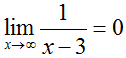
In this graph, it is fairly piece of cake to encounter that as x becomes increasingly large or increasingly modest, the y-value of f(x) becomes very shut to zero, though information technology never truly does equal goose egg. When a role'due south curve suggests an invisible line at a certain y-value (such every bit at y=0 in this graph), it is said to accept a horizontal asymptote at that y-value. Nosotros tin can use limits to describe the behavior of the horizontal asymptote in this graph, every bit:

and

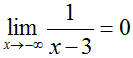
Try setting xmin as -100 and xmax as 100, and yous will come across that f(x) becomes very shut to zero indeed when x is very large or very modest. Which is what you should wait, since one divided past a large number volition naturally produce a pocket-size result.

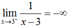
The concept of i-sided limits can be applied to the vertical asymptote in this example, since i can see that as x approaches iii from the left, the part approaches negative infinity, and that as x approaches 3 from the right, the function approaches positive infinity, or:

and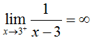

Unfortunately, the beliefs of functions as x approaches positive or negative infinity is non e'er so piece of cake to describe. If always y'all see a case where you can't discern a function'southward beliefs at infinity--whether a graph isn't available or isn't very clear--imagining what sort of values would be produced when ten-chiliad or 1-hundred yard is substituted for 10 will normally requite you a good indication of what the office does as x approaches infinity.

Powers and Exceptions

Let's analyze a couple of not-so-straightforward examples apropos limits at infinity to ensure a total understanding of how they work. Take a look at this strangely bird-like role:

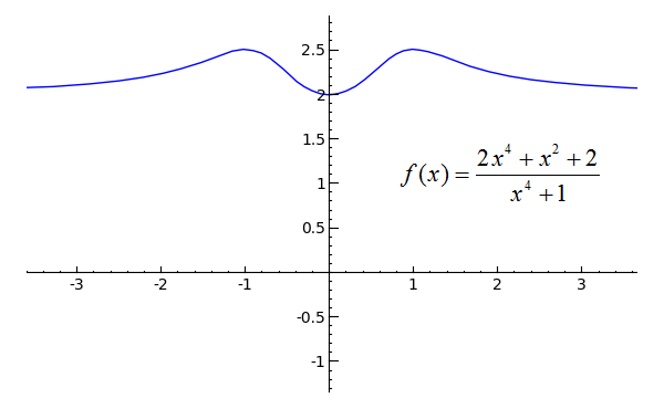
plot((2*10^4 + x^2 + 2)/(x^four + i), x, -4, 4).show(xmin=-3, xmax=three, ymin=-one, ymax=two.5)

Toggle Line Numbers

The graph gives information technology abroad; the limit of the function as x approaches either positive or negative infinity is two. But what if we didn't take the graph? There are actually a couple of clues as to what value the function approaches at both infinities. Compare the numerator to the denominator: see how the "highest ability" of each polynomial is 4? The numerator has 2*x⁴ and the denominator has simply x⁴. Perhaps y'all see where this is going--what do you become when you separate 2*ten⁴ by x^iv? Why, two of grade. But put, when the numerator and the denominator of a office take the same ability--when the highest exponents of x between the top and bottom of the fraction lucifer--the office will take a horizontal asymptote at y equals (coefficient of numerator's highest power) / (coefficient of denominator'south highest power).

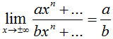
Well...mayhap that wasn't so simple. Permit me reiterate with a general case. For a function similar this 1:

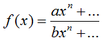
Assuming that due north is the highest exponent of both the numerator and denominator and that a and b are coefficients:

For this trick to work, though, the function must be a rational expression (one polynomial divided past some other) and cannot take trigonometric or other special functions in the numerator or denominator. For example, the horizontal asymptote of the following function cannot be found using the above method, as information technology refers to an expression where x is an exponent.

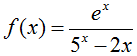
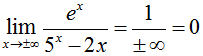
Earlier you graph this function to see if and where information technology has a horizontal asymptote, though, let united states of america try a fleck of logical analysis. First, which will grow the fastest, due east^10 or 5^ten? Evaluating 'float(due east)' in SageMath will tell you that Euler'south number e equals approximately 2.7182818284590451, then 5^10 volition grow more quickly than e^10. But what about the 2*10 in the denominator? Consider the growth, now, of five^x relative to two*x. When x is 5, the former evaluates to 3125 while the latter evaluates to 10. What you should gather from this is that five^ten trumps all; as x approaches positive or negative infinity, the function will become the quotient of a big number (e^ten) divided by a really big number that only continues to grow. In other words, one could write this as:

And tada! There you have it. Comparing relative growths is another way of figuring out the beliefs of a office as its independent variable approaches infinity. Keep reading to larn nigh this lesson's final type of function, those that oscillate.

Oscillating Functions

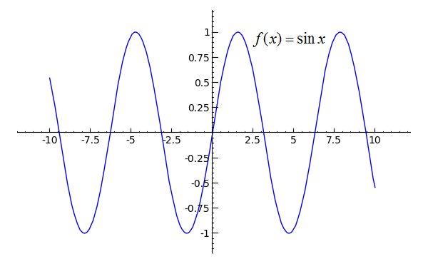
plot(sin(x), x, -10, 10)

Toggle Line Numbers

Like nearly of the trigonometric functions, as x approaches positive or negative infinity, the sine function itself continues to spring up and down. An aquiver part is i that continues to motion between two or more values as its independent variable (ten) approaches positive or negative infinity. The limit of an aquiver function f(x) as x approaches positive or negative infinity is undefined. In the plot that you simply created, endeavour replacing 'sin' with diverse other trigonometric functions such as 'cos', 'tan', 'sec', 'csc', 'cot', or any of the arc-functions (like 'arctan') to observe whether they oscillate or whether they have a horizontal asymptote as x approaches positive or negative infinity.

The adjacent graph behaves differently though, as y'all may observe:

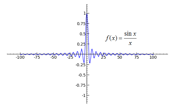
plot(sin(10)/x, ten, -100, 100).prove(ymin=-1)

Toggle Line Numbers

Even though the function oscillates indefinitely due to the sine function in its numerator, I can tell y'all without a dubiety that the limit of the function as x approaches either positive or negative infinity is nonetheless zero. But why is this? The sine of a really big number must however exist somewhere in the range of -1 and 1, while denominator will but be a really large number. If we create a tabular array of values, we can lookout the role's behavior when x is large. Utilise the following code to create such a table.

def f(10):     render sin(ten) / x  def table():     print('|   x   |   f(ten)    |')     print('|-------------------|')     for ten in [10000..10010]:         print('|%6i | %+f |'%(x, f(x)))  tabular array()

Toggle Explanation Toggle Line Numbers

1-2) Ascertain a function f(x) that is equal to sin(x)/10. The 'def f(x):' signifies "when f(x) is referenced, do whatever the next indented line says".
four) Define a part called 'table'
5-half-dozen) Print the header of the table.
7) Starting at x=10000, perform the following indented command, incrementing x by i every fourth dimension.
8) Impress the electric current values of x and f(10). '%6i' means "fill vi spaces with the post-obit integer", while '%+f' means "put a positive or negative sign in front of the following floating signal number". The '%(x, f(x))' at the terminate of the line tells SageMath which numbers to use when information technology replaces the preceding percentage signs.

There is another mode to testify that the limit of sin(x)/x as 10 approaches positive or negative infinity is zero. Whether y'all have heard of it equally the pinching theorem, the sandwich theorem or the squeeze theorem, every bit I volition refer to it here, the squeeze theorem says that for 3 functions g(x), f(10), and h(x),

If 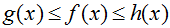and ,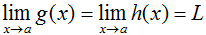
then .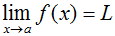

To apply this theorem, nosotros accept to observe a function g(x) that is less than f(x) as well every bit a role h(x) that is greater than f(x). Since sin(x) is always somewhere in the range of -1 and 1, we can set chiliad(ten) equal to -1/x and h(x) equal to 1/x. We know that the limit of both -1/ten and 1/x as 10 approaches either positive or negative infinity is zero, therefore the limit of sin(ten)/ten as x approaches either positive or negative infinity is zero. I could write this out as:

Given that and ,
since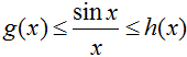 for all x in and ,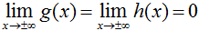
information technology follows that .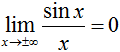

Practice Problems

Notice the limit of each part as x approaches positive and negative infinity, if either exists. Endeavour determining each limit by analysis and/or plotting, then cheque your results in the Notebook using 'limit(..., ten=...)'.
1)     Toggle answer
2)     Toggle answer
3)     Toggle respond